Add Drop Down in Excel: How to Create and Manage Drop Down List in Excel

MS Excel is full of amazing features, Drop Down is one of them which can come in handy for more accuracy.

Published On: Apr 12, 2023

A drop-down menu is a great feature implemented by Microsoft in Excel. It can be a huge help when you are working with multiple people at once and you want them to enter the correct data in the cell. By setting up a drop-down menu, you can make sure that the data and value that gets entered are correct every time. There are several ways you can set up a drop-down in Excel.

By setting up a dropdown in the Excel cells, you can make repetitive tasks like student attendance, employee data and your regular expenses easy. It also decreases the chances of making errors in the data by giving the correct values as choices. I have covered the methods to set up dropdowns in Excel for different platforms like macOS, Windows and Excel Online.

Table of Contents

How to Create a Drop-Down List in Excel

There are various methods to get it done based on which operating system you are trying to get it done. You can scroll below to see the process for the operating system you are on.

How to Create Drop-Down in Excel on Windows

Excel is a native app from Windows and comes preinstalled on almost every Windows desktop. If you are also using this and want to implement the drop-down in Excel, you can follow the below steps to get it done.

First thing first, make a table on the other Excel page. Select a new page from the bottom ribbon and press Ctrl+T to make the lists that you want in the drop-down. Making a table of data makes it easier for Excel to fetch data in the drop-down.

Select the Cell where you want to imply the drop-down
From the tools tab, select the Data menu
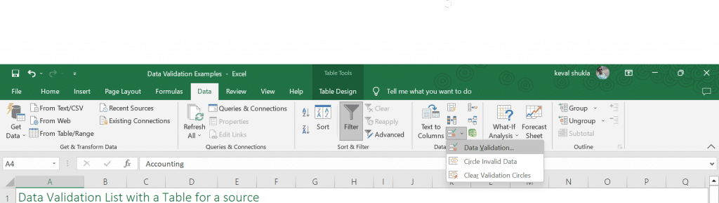
Click on data validation
From the pop-up, select the Settings option
In the “Allow”, select the Lists option
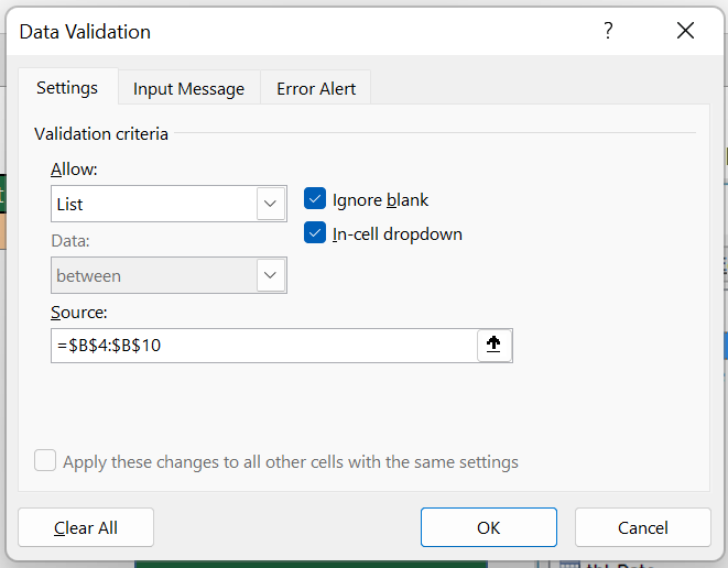
Select the Source field
Select the Table of list you want in the drop down
Mark a checkbox called “Ignore Blank” if you don’t want an empty field, otherwise leave it unchecked
Check option called “In cell dropdown box”
Click OK

Input message tab

An input message is shown when the user clicks on the cell. It’s used when you want to give certain instructions when the Excel cell is clicked to select an option from drop-down. If you want to display a message or set of instructions inside a drop-down cell, continue the steps, or you can skip to the next instructions.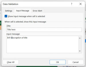

Select the Input message tab once you are done with lists in Dropdown
Check the box called “Show message when the cell is selected” if you want to display a message only when the user clicks on a cell.
Now enter the Title in the title field
Enter the title description in the below field
Click OK once you are done

Error Alert tab

As the name explains itself, when you insert the wrong data inside the list cell, it pops up with an error message. You can customize this message as per your requirement if you want.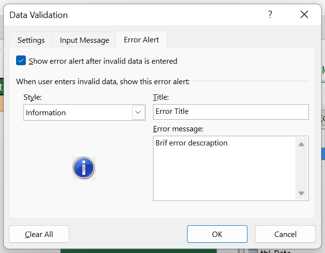

Check box to shadow alert after user enters invalid data
Select style, how you want your message to be displayed
Tip: Keep the style as “Informative” where it’s possible to prevent users from skipping to insert value after getting error message.
After choosing style, select the title field which will be displayed
Under the title, enter the brief description of the given title

How to Create Drop-Down in Excel on macOS

If you are using Excel on macOS-based devices and you want to add a drop-down option in your cells, then this one is for you. Follow the given steps to add the drop-down in the cells.

Using a sheet with a single column or row without blank cells, create a list of valid entries for the dropdown list
Make sure the cells you want to restrict data entry are selected
Choose Data Validation from the Tools ribbon under the Data Validation menu.
Under the Settings tab, select Allow from the Allow pop-up menu.
Now select the List inside Allow pop up
Under the lists option, select the Source input field
Select the list of entries you created in the first step
Press the Return or OK button to save your settings

You are now done with the Drop Down list in your Excel cells on your Mac devices.

How to Create Drop-Down in Excel on Web

If you are using the Web version of Excel and want to set up a drop-down, then look no more. Here’s how you do it.

This will work on any operating system, as the web version is the same for everyone.

Open a new page in your worksheet and create a table of lists with a single column of the items you want in the drop-down
Go to your main worksheet and select the cell you want to add dropdown
After selecting the cell, select Data from the toolbar ribbon
From the Data menu, select Data validation
On settings, inside Allow popup, select list
Now, In the source field, select the table you created earlier from the second sheet page
Check the Box called “Ignore Blank” if leaving the cell is empty is ok
Now fill up the Message you want to be displayed in the Input message tab
Next to the Input Message tab, select the Error Alert tab and set the title and description for when the user makes an error while inserting data
Click ok it will save the settings

This is how you can easily add in the drop-down in any of your Excel worksheets. It makes it far better and more time efficient, and in addition, it rescues the chances of eros in data.

How to Create Drop-Down List in Excel With Multiple Selections

When you want to select more than one data in the cell from the Drop Down, you can use multiple selections. There are a few different ways you can use to select multiple options inside the Drop Down. the easiest way to achieve it is to use Kutools for excel, and another way is tinkering with the VBA code in MS Excel.

How to Add Multiple Selections in Excel Drop Down Using Kutool

Download and install the Kutools addon
Restart the MS Excel and go to the Excel sheet with the drop-down you want to set multiple selections.
Select the cell with Drop down on it, and then from the toolbar ribbon, select the KuTools tab and then select Drop Down list option.
From the pop-up menu, Select multi-drop-down lists and enable it.

Using the extension, it’s as easy as that you can also go to its settings and enable or disable the settings if you don’t want the duplicate values or you want the duplicate values.

How to Add Multiple Selections in Excel Drop Down by Editing VBA Code

Now to enable multiple selections using the VBA Code, you need to play with the coding part of the Excel sheet. It might look complex, but once you do the process step by step, you will feel otherwise.

There are two different codes to enable multiple selections inside the Drop Down cell. One to enable multiple selections without allowing the duplicate selection on. Another one which also does not allow the user to choose a duplicate selection, but when the user makes a duplicate selection, it deletes the selected entry. Follow the steps to understand how to add the VBA Code to the Excel Sheet

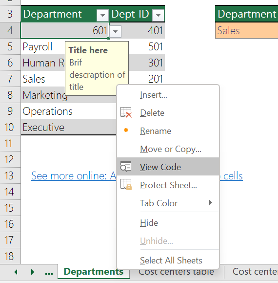
Open the worksheet with Drop Down in it
In the bottom SHeet tab right, click o the Sheet name and select View code from the pop up menu
Inside Microsoft Visual Basic for application past the given code in the workbook code field
Once you paste the code, change the values as instructed at begining of code
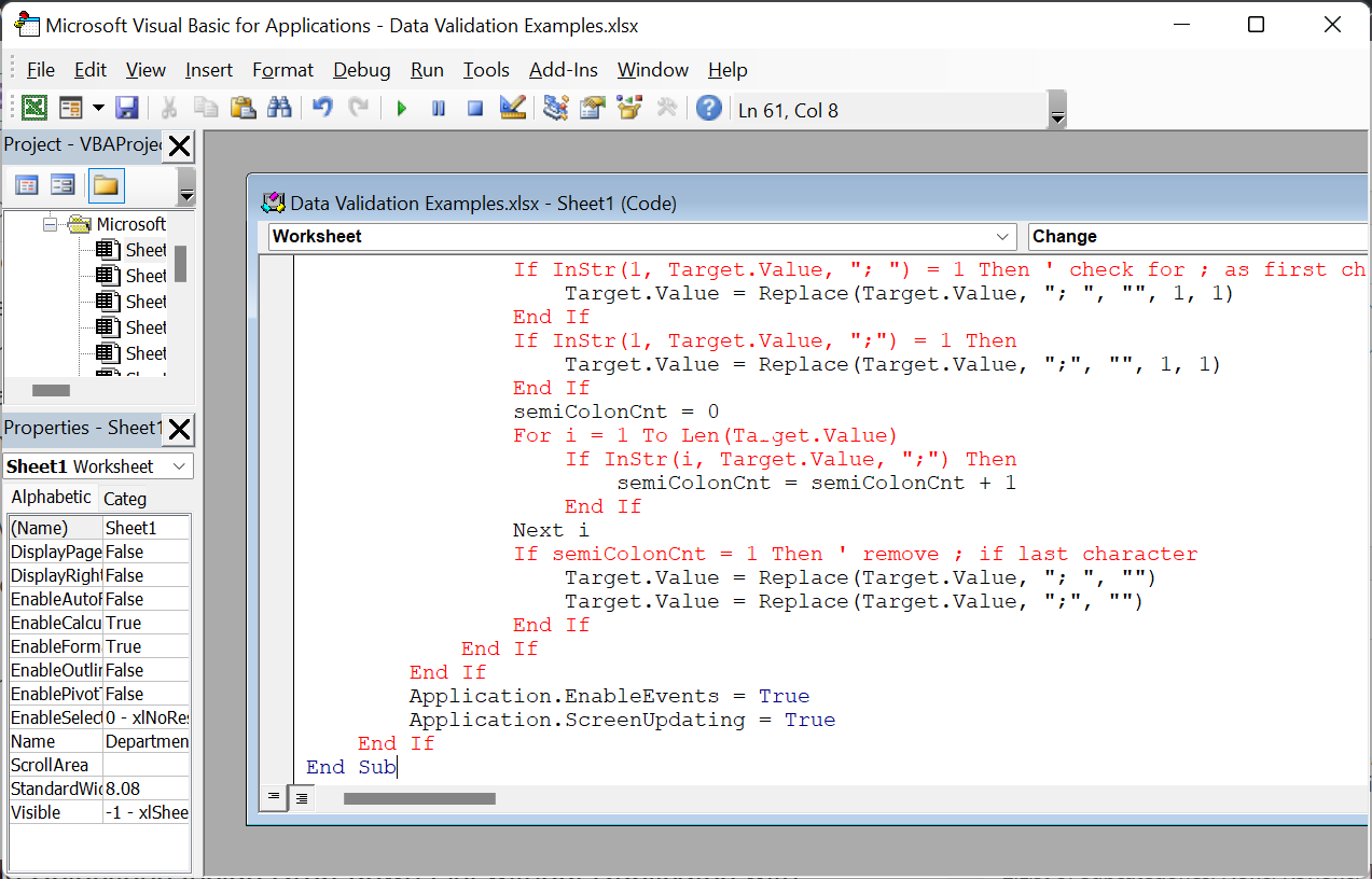
Click enter and close the window

Allow Multiple Selections Inside Drop-down List without Duplicates with Deletable Entry

Private Sub Worksheet_Change(ByVal Target As Range)
Dim xRng As Range
Dim xValue1 As String
Dim xValue2 As String
Dim semiColonCnt As Integer
Dim xType As Integer
If Target.Count > 1 Then Exit Sub
On Error Resume Next
xType = 0
xType = Target.Validation.Type
If xType = 3 Then
Application.ScreenUpdating = False
Application.EnableEvents = False
xValue2 = Target.Value
Application.Undo
xValue1 = Target.Value
Target.Value = xValue2
If xValue1 <> “” Then
If xValue2 <> “” Then
If xValue1 = xValue2 Or xValue1 = xValue2 & “;” Or xValue1 = xValue2 & “; ” Then ‘ leave the value if only one in list
xValue1 = Replace(xValue1, “; “, “”)
xValue1 = Replace(xValue1, “;”, “”)
Target.Value = xValue1
ElseIf InStr(1, xValue1, “; ” & xValue2) Then
xValue1 = Replace(xValue1, xValue2, “”) ‘ removes existing value from the list on repeat selection
Target.Value = xValue1
ElseIf InStr(1, xValue1, xValue2 & “;”) Then
xValue1 = Replace(xValue1, xValue2, “”)
Target.Value = xValue1
Else
Target.Value = xValue1 & “; ” & xValue2
End If
Target.Value = Replace(Target.Value, “;;”, “;”)
Target.Value = Replace(Target.Value, “; ;”, “;”)
If Target.Value <> “” Then
If Right(Target.Value, 2) = “; ” Then
Target.Value = Left(Target.Value, Len(Target.Value) – 2)
End If
End If
If InStr(1, Target.Value, “; “) = 1 Then ‘ check for ; as first character and remove it
Target.Value = Replace(Target.Value, “; “, “”, 1, 1)
End If
If InStr(1, Target.Value, “;”) = 1 Then
Target.Value = Replace(Target.Value, “;”, “”, 1, 1)
End If
semiColonCnt = 0
For i = 1 To Len(Target.Value)
If InStr(i, Target.Value, “;”) Then
semiColonCnt = semiColonCnt + 1
End If
Next i
If semiColonCnt = 1 Then ‘ remove ; if last character
Target.Value = Replace(Target.Value, “; “, “”)
Target.Value = Replace(Target.Value, “;”, “”)
End If
End If
End If
Application.EnableEvents = True
Application.ScreenUpdating = True
End If
End Sub

Allow Multiple Selections Inside Drop-down List Without Duplicates

Private Sub Worksheet_Change(ByVal Target As Range)
Dim xRng As Range
Dim xValue1 As String
Dim xValue2 As String
If Target.Count > 1 Then Exit Sub
On Error Resume Next
Set xRng = Cells.SpecialCells(xlCellTypeAllValidation)
If xRng Is Nothing Then Exit Sub
Application.EnableEvents = False
If Not Application.Intersect(Target, xRng) Is Nothing Then
xValue2 = Target.Value
Application.Undo
xValue1 = Target.Value
Target.Value = xValue2
If xValue1 <> “” Then
If xValue2 <> “” Then
If xValue1 = xValue2 Or _
InStr(1, xValue1, “, ” & xValue2) Or _
InStr(1, xValue1, xValue2 & “,”) Then
Target.Value = xValue1
Else
Target.Value = xValue1 & “, ” & xValue2
End If
End If
End If
End If
Application.EnableEvents = True
End Sub

How to Create Drop-Down List but Show Different Values In Excel

After quickly creating the Drop Down list, you can try to show a different value when you select the value in the drop down list. Like for example, when you select a student’s name from the drop down it prints the roll number in the cell instead of the name.

To achieve this, first, you need to create the table with two columns, one with the list value and the second with print value, unlike previously, where you only create a table with one value in it for drop down. Now after finishing off with the preparation, follow these steps to get it done.

Select the Name value and create the usual drop down list following steps mentioned above
After making the dropdown list right, click on the sheet name on bottom sheets page
From the pop up, select View code
Once the Visual Basic Code application opens, paste this VBA code into it,
Private Sub Worksheet_Change(ByVal Target As Range)

selectedNa = Target.Value

If Target.Column = 5 Then

selectedNum = Application.VLookup(selectedNa, ActiveSheet.Range(“dropdown”), 2, False)

If Not IsError(selectedNum) Then

Target.Value = selectedNum

End If

End Sub

Once you paste the code replace “Dropdown” with the Range of column. If you want to select columns from C2 to C8 then it can be written like C2:C8

How To Edit Drop-Down List In Excel

To edit the items in the drop down lists in Excel,

Go to the table where you have listed the value
Add the new value at the bottom of the list or remove the value and clear the empty space
Select the cell with Drop Down list
Go to the Data menu from the toolbar ribbon, then click on data validation
Now Edit the Vaalues according to new lists like the cells from where it fetches the values

As simple as that, you can easily edit the Drop Down in the Excel worksheets.

Frequently Asked Questions

1. How do I colour code a drop-down list in Excel?

Once you create the Drop Down lists, go and select the table of lists, then go to Home then select Conditional Formatting and thereafter select the option called New Rule. Inside the New Formatting rule pop-up, select the option that says “Select only cells that contain”.

After selecting that inside the rule description field, Select Format only Cells With and set values for your text for the cell. There will be multiple tabs like Number, Font, Border, and Fill. After setting up the rule, click OK.

2. Is there any formula for excel drop down list

Yes, you can use multiple different formulas depending on your need to create a drop-down in cell. You can use the If function inside the table Cell to create the drop down based on the selected table content. To create a dependent dropdown based on the selected cells, use the INDIRECT Function. And lastly, use the VLOOKUP function for the formula-based dropdown list.

3. Is a drop-down list the same as data filtering?

No, a Dropdown is a type of list that lets you choose your preferred values from your selected list of values, while data filtering is a way to display data that matches certain criteria.