VLOOKUP Formula: What is It, How To Use VLOOKUP in Microsoft Excel with Example

Here is how you can use the VLOOKUP formula in MS Office.

Published On: February 19, 2022

JOIN US

Microsoft Excel or MS Excel is one of the most powerful tools when it comes to managing, filtering, and exploring data. The spreadsheet software developed by Microsoft is being used by millions of users on Mac, Windows, Android, and iOS on a regular basis. MS Excel offers computational capabilities, graphing tools, visualization tools, and more.

With features like formula and features, Excel can handle anything you throw at it in terms of calculations. Things get interesting once you start using formulas and one such formula on the MS Excel platform is the VLOOKUP formula.

In this article, we will take a look at what is a VLOOKUP formula and why it used. We will also take a look at how the formula can be used with some examples and syntax.

Also Read: MS Excel Shortcut Keys: Best Microsoft Excel Keyboard Shortcuts for Windows and macOS Computers

Table of Contents

What is VLOOKUP Formula in Excel and Why is it Used?

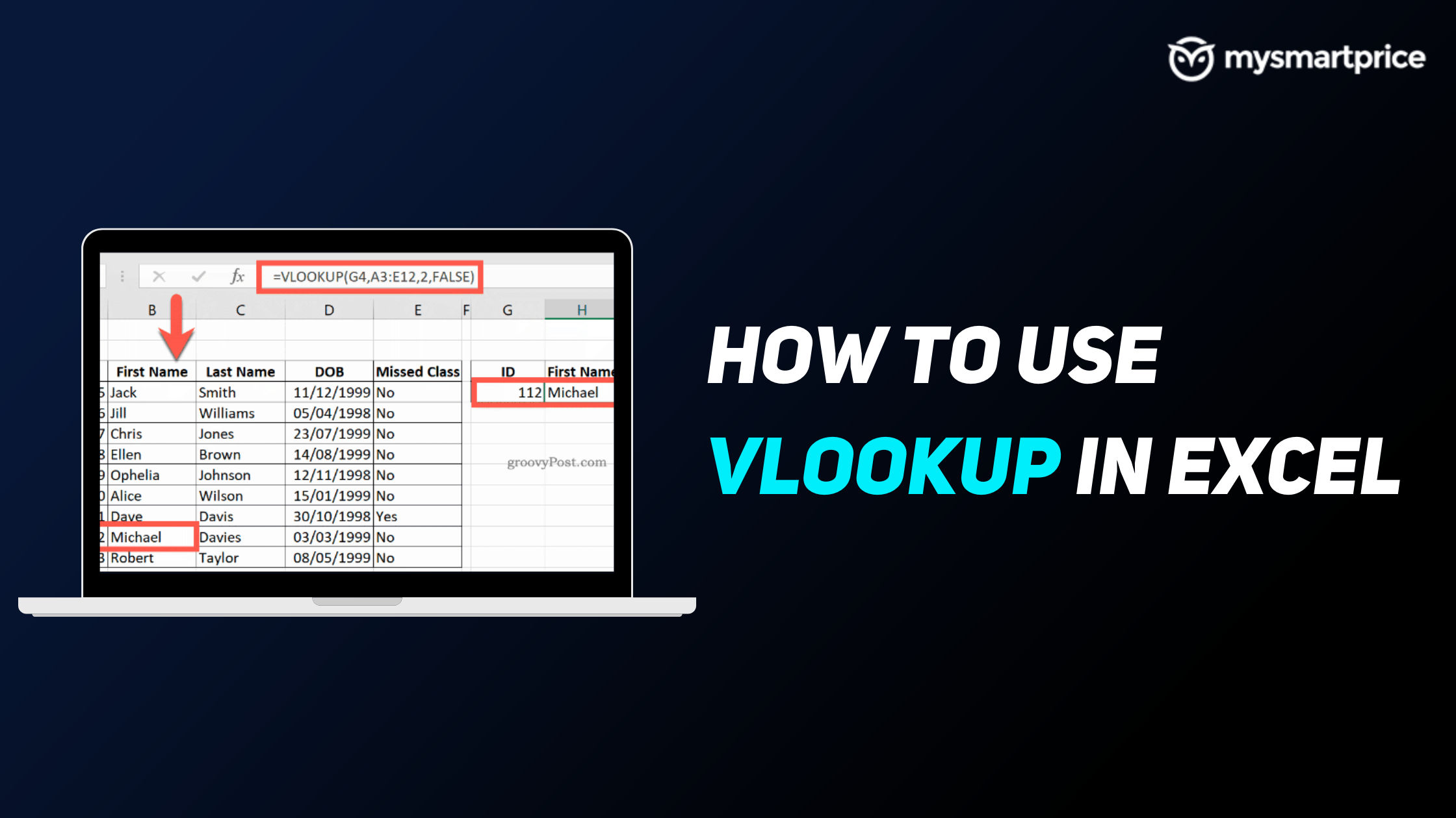
VLOOKUP is a pretty handy and powerful formula in MS Excel and it is also one of the most widely used formulas to save time and effort. For starters, the VLOOKUP stands for vertical lookup. This formula is used when you have to find things in a table or a range by row. It searches down the first column of a range for a key and returns the value of a specified cell in the row found.

Here is the simple form to use the VLOOKUP formula:

=VLOOKUP(What you want to look up, where you want to look for it, the column number in the range containing the value to return, return an Approximate or Exact match – indicated as 1/TRUE, or 0/FALSE)

Examples:

=VLOOKUP(1003, A2:B26, 2, FALSE)
=VLOOKUP(A4,A10:C20,2,TRUE)
=VLOOKUP(“Steve”,B1:E7,2,FALSE)
=VLOOKUP(A2,’Client Details’!A:F,3,FALSE)

Also Read: MS Word Shortcut Keys: Full List of Keyboard Shortcuts for Windows and macOS Laptops or PCs

How to use VLOOKUP Formula in Excel

Now that you have seen some of the examples above, here is the syntax to use the VLOOKUP formula in Excel.

Syntax: VLOOKUP (lookup_value, table_array, col_index_num, [range_lookup])

Let’s understand what the arguments inside the brackets mean and if they are mandatory and what value needs to be filled in while using it.

lookup_value (mandatory)

Here you need to enter the value you want to look up/search for. The value you want to look up must be in the first column of the range of cells you specify in the table_array argument. It can be a value or a reference to a cell.

Example: If table-array spans cells B2:D7, then your lookup_value must be in column B.

table_array (mandatory)

The second mandatory field that you need to enter, table_array refers to the range of cells in which the VLOOKUP function will search for the lookup_value and then gets back the value. You can use a named range or a table, and you can use names in the argument instead of cell references. The first column in the cell range must contain the lookup_value. The cell range also needs to include the return value you want to find.

col_index_num (mandatory)

The column number, which contains the return value. The number starts with 1 for the left-most column of table_array.

range_lookup (optional)

This optional field takes a logical value that specifies whether you want VLOOKUP to find an approximate or an exact match. You can enter 1/TRUE to find an approximate match. This assumes the first column in the table is sorted either numerically or alphabetically, and will then search for the closest value. This is also the default method in case you don’t enter anything manually.

Example: VLOOKUP(90,A1:B100,2,TRUE)

To get the exact match, you can use 0/FALSE, which searches for the exact value in the first column

Example: =VLOOKUP(“Smith”,A1:B100,2,FALSE)

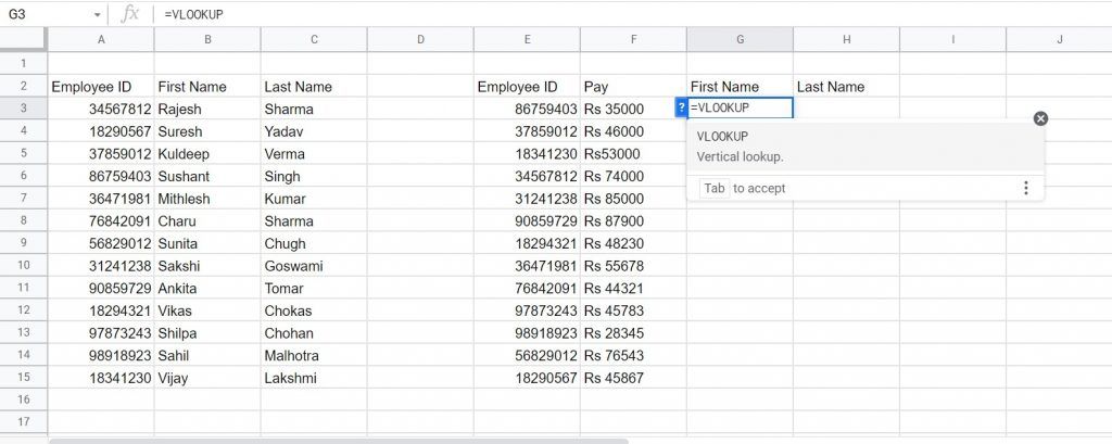
Pro Tip: To build the VLOOKUP syntax quicker, write “=vl” and then hit enter the tab key to autocomplete the formula name.

Now that we have understood how and when to use the VLOOKUP formula, let’s take a look at a real-life example.

Open the spreadsheet with data where you want to use the VLOOKUP formula
Click on the cell where you want to execute the VLOOKUP formula
Enter =VLOOKUP(
Enter lookup value you want to get
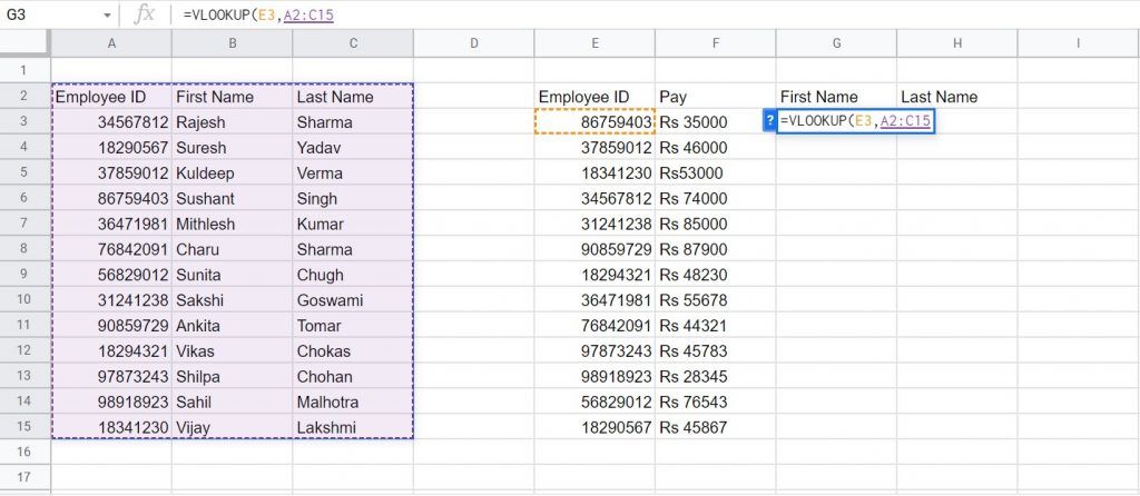
Enter the range of cells in which the VLOOKUP will search for the entered value
Next, enter the col_index_num in which we want to find the lookup value and the return value.
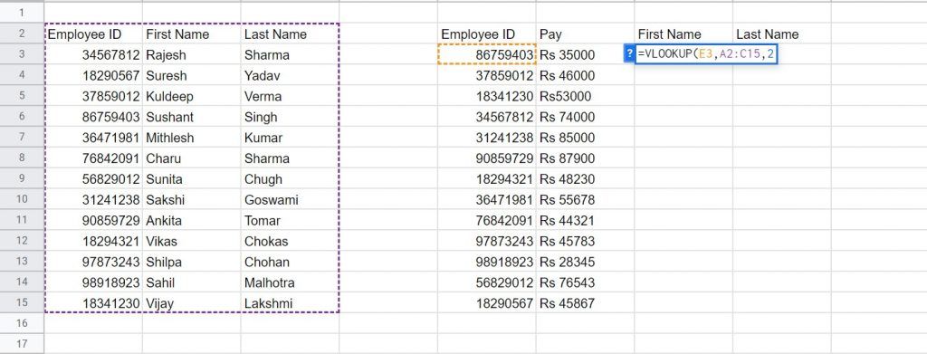
Lastly, enter 1/TRUE to get an approximate match or 0/FALSE to find the exact match
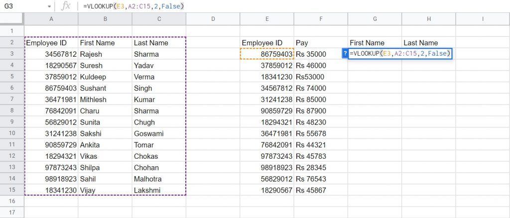
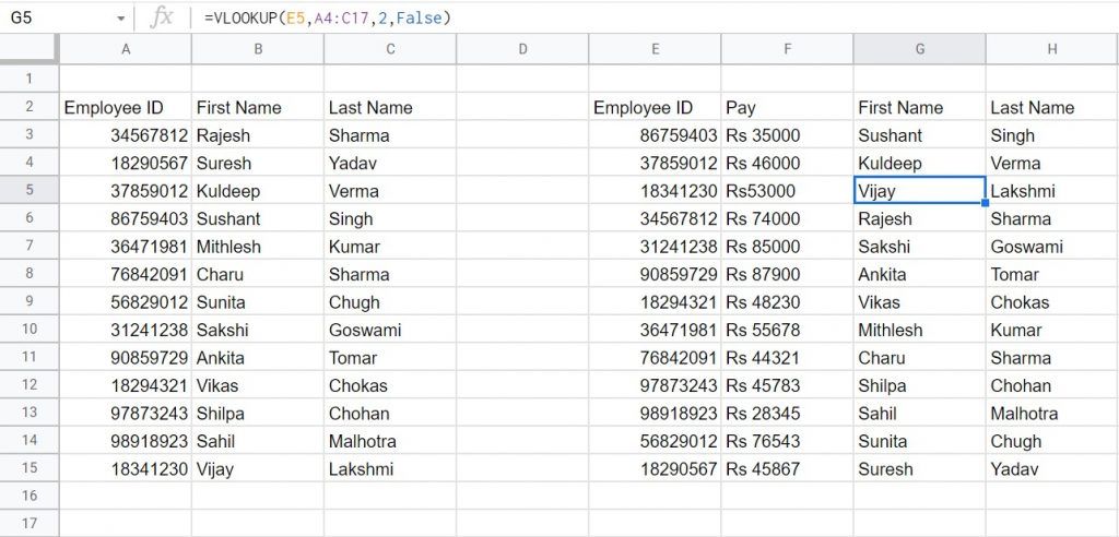
Hit enter and you will get the result containing the value you were looking for in the earlier step