Microsoft Excel is the go-to tool for working with data. Excel can seem like a simple tool for writing down data in an orderly form, but it is a much more advanced and powerful spreadsheet program.
You can perform complex calculations, in-depth charts, graphs, and more. Empowering you to do all these are Excel formulas. You can do any type of simple and complex calculations with Excel formulas. In this article, we talk about the top Excel formulas. We have listed the best and top formulas according to basic, intermediate, and advanced formulas and according to their functions. Read on!
What Are Excel Formulas?
Excel formulas in Microsoft Excel are an expression that operates on values on a single cell or a range of cells. Formulas can perform different calculations such as addition, subtraction, multiplication, division, and more. These are the simple Formulas; there are also intermediate and advanced formulas, which are used to perform more complex calculations using Excel.
All the Formulas come with a similar structure. They all start with an equal sign, ‘=,' and are followed by the formula or function and then operators. Excel calculates from left to right and uses PEMDAS (Parentheses, Exponents, Multiplication, Division, Addition, Subtraction) in order of operations.
How To Insert Formulas In Excel?
Here's how to create a formula in Microsoft Excel:
- Select a cell.
- Type the equal sign ‘=’ first.
- Select a cell or type the address of the cell in the selected cell.
- Enter an operator. For example, – for subtraction.
- Type the address of the second cell or select the cell.
- Press Enter, and the result of the formula will be shown in the selected cell with the formula.
Basic Excel Formulas
SUM
The SUM() formula adds data on the selected cells. It works on cells with numerical data and requires two or more cells to perform.
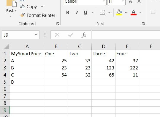
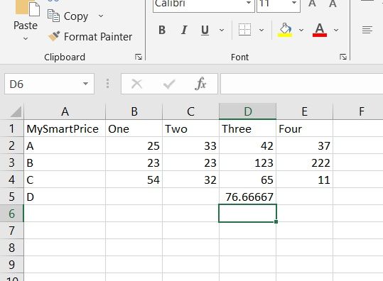
For example, take a look at the above-given sheet. If I want to add the cells D2 to D4 and display the result of that in the D5 cell, the SUM formula for it will be:
- =SUM(D2:D4)

You can either type the cell numbers (D2, D3, D4), provide the range of cells (D2:D4), or drag and select the cells.
AVERAGE
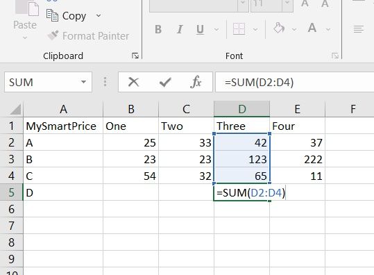
The AVERAGE() formula finds out the average of the data on the selected cells.
In the same example as before, if you want to make out the average of the cells from D2 to D4, you can either provide the range of cells (D2:D3) or you can select individual cells (D2, D3, D4)
The formula for the Average will be:
- =AVERAGE(D2:D4)
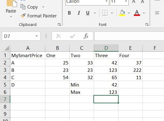
MIN and MAX
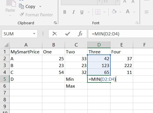
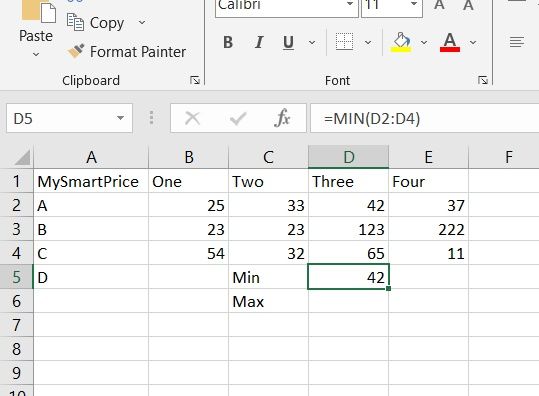
The MIN() formula finds out the minimum number in the select range of cells.
Let's find the minimum among the three numbers in the selected range in the same example as before. The formula for that will be:
- =MIN(D2:D4)
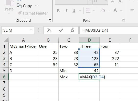
The MAX() formula does the direct opposite of the MIN formula, finding the maximum in the select range of cells. The formula for this would be:
- =MAX(D2:D4)
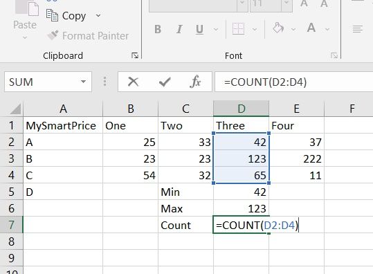
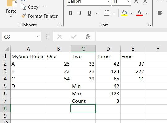
COUNT
The COUNT() formula counts the total number of cells in the selection. It will not count blank cells or data formats other than numeric. Here's the count formula for the same example as above:
- =COUNT(D2:D4)
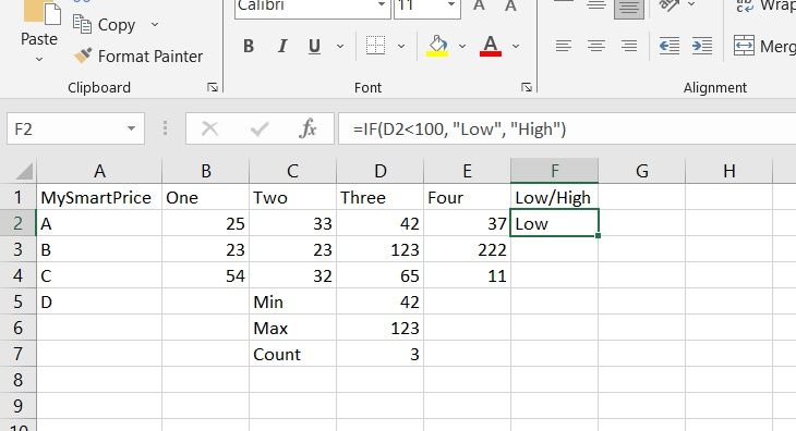
IF
The IF() formula is like the simple if-else statement in programming languages. This function can classify a data set according to the if-else logic.
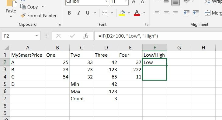
Let’s take the same example. Consider I want to highlight the numbers above 100 as High and the numbers below 100 as Low; this is the formula to use:
- =IF(D2<100, "Low", "High")
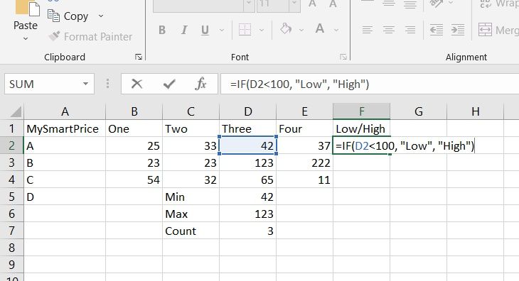
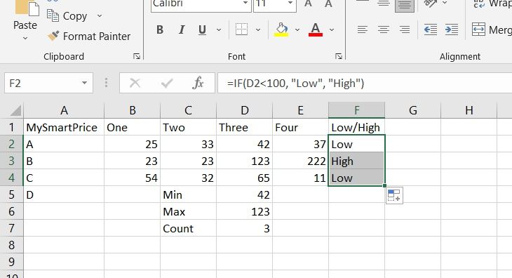
You can select and drag the cell with the result to apply the formula to all the cells below.
Intermediate Excel Formulas
VLOOKUP
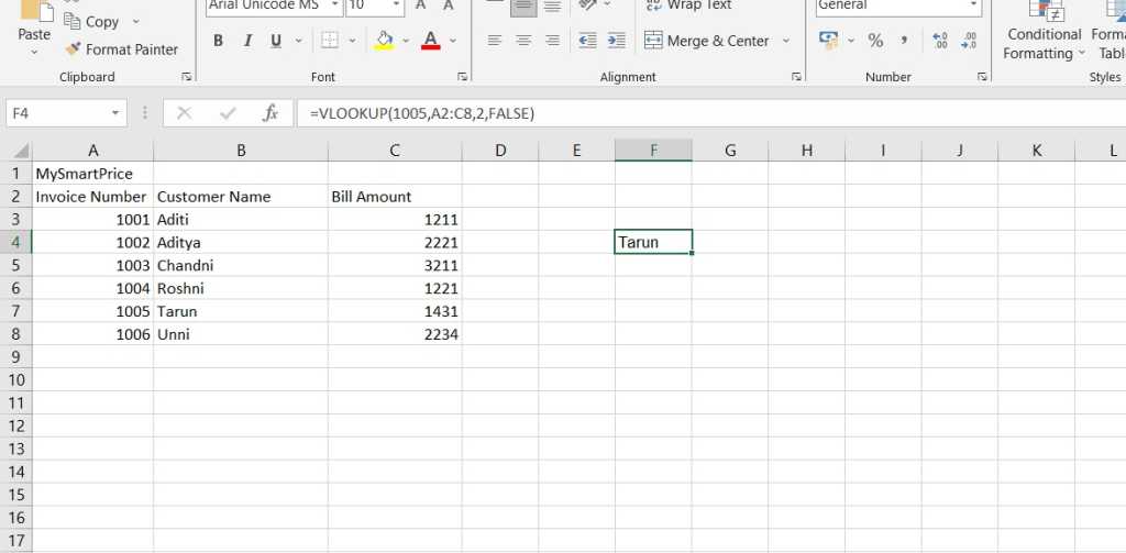
VLOOKUP stands for Vertical Lookup, and it helps you look for data vertically across the sheet. For example, you have an invoice number, and various data is vertically added along the invoice number in the horizontal cells. You can use the VLOOKUP formula to find the value in the corresponding column.
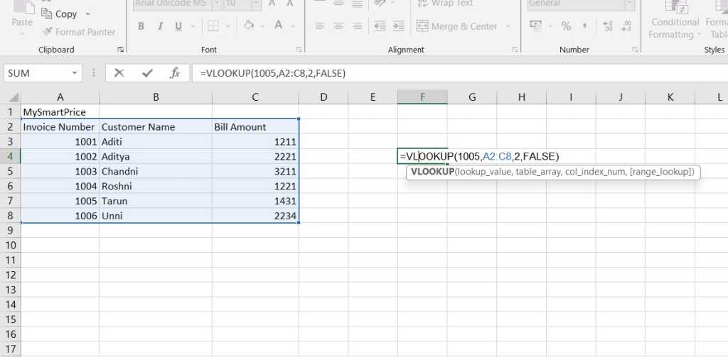
Here's the formula for VLOOKUP:
- =VLOOKUP(lookup_value, table_array, col_index, range_lookup)
And here's what each term means:
- lookup_value: The value you're looking for in the first column.
- Table_array: The range of the values you're looking up.
- col_index: The position of the column to extract the value from.
- range_lookup: "TRUE" for approximate match (default), and "FALSE" for exact match.
In the below example, we look for the corresponding name for the invoices:
HLOOKUP
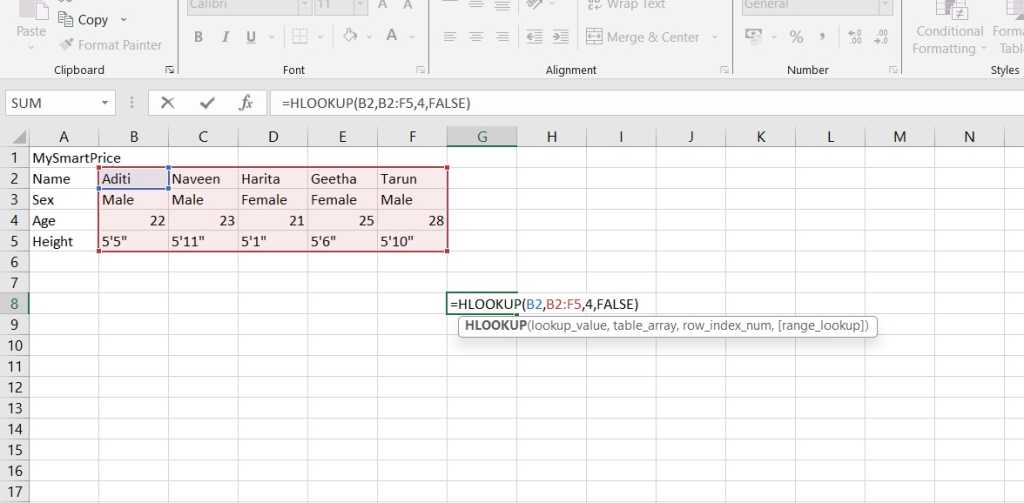
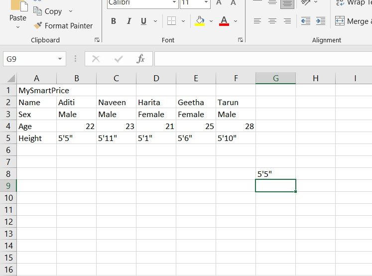
HLOOKUP stands for Horizontal Lookup, and it is similar to VLOOKUP, but horizontally across the sheet.
Here's the HLOOKUP formula:
- =HLOOKUP(lookup_value, table_array, row_index, range_lookup)
Here is what each term stands for:
- lookup_value: The value you're looking for in the first row.
- Table_array: The range of the values you're looking up.
- col_index: The position of row to extract the value from.
- range_lookup: "TRUE" for approximate match and "FALSE" for exact match.
In the example below, let's check out the sex of the students:
SUMIFS
SUMIF performs addition based on the sum of a range of numbers.
Here's the SUMIFS formula:
- =SUMIFS(sum_range, criteria_range1, criteria1, [criteria_range2, criteria2] …)
The conditions for addition is represented as criteria 1, criteria2, etc. It can check these such as:
- > – If the number is greater than.
- < – If the number is less than.
- = – If the number is equal to.
The [sum_range] is the range for the function to calculate the sum.
COUNTIFS
The COUNTIFS formula is used for counting cells that fall under a specific criteria or condition.
Here's the structure of COUNTIF formula:
- COUNTIF(range, criteria)
The two arguments are defined as below:
- range – This defines the cell or cells to count.
- criteria – This defines the cells the function needs to count.
A simple use of this formula is to count the number of times a name or value appears in a column.
TRIM
The TRIM formula is used to remove irregular spaces in a data set.
Here's the TRIM formula:
- =TRIM(range)
You just have to use the TRIM formula with the range of cells. It will return a separate dataset with irregular spaces removed.
Advanced Excel Formulas
OFFSET
The OFFSET function returns a cell or range of cells specified using the OFFSET formula.
Here's the OFFSET formula:
- =OFFSET(reference, rows, cols, [height], [width])
These are what the arguments mean:
- Reference – The cells or range of cells to base the offset.
- Rows – The number of rows to move from the starting point.
- Column – The number of columns to move from the starting point.
- Height – The number of rows to return (optional)
- Width – The number of columns to return (optional)
IF AND
The IF AND formula combines the IF and AND functions in a single formula. With the IF AND formula, you can return one result for meeting the set of conditions and another result for failing to meet the conditions.
Here's the formula for IF AND:
- =IF(AND(condition1, condition2, value_if_true, value_if_false)
This can be seen as an extension of the IF formula we discussed in the basic Excel formulas list. There's a second condition instead of one in the formula. Given above as condition 1 and condition 2. You can give the values of true and false based on these conditions.
IF OR
The IF OR formula combines IF and OR functions into a single formula. It works similarly to the IF AND formula, which returns true or false values based on meeting these conditions.
Here's the formula for IF OR:
- =IF(OR(condition1, condition2, value_if_true, value_if_false)
If it meets the two conditions, given as condition1, condition 2, the value_if_true and value_if_false are where you give the values to be shown if the conditions are met or if they haven't.
INDEX
With the INDEX formula, you can return a value from a list of values based on its index number in the cells.
Here's the INDEX formula:
- =INDEX(array, row_num, [column_num])
This is what each of the items means:
- Array – The range of cells.
- Row_num – The row number in the selected array of cells to return the value.
- Column_num – The column number in the select array of cells to return the value.
IFERROR
The IFERROR formula is used to manage errors in calculations and formulas. IFERROR function checks if a formula is correct, evaluates the error, and returns another value you can specify.
Here's the IFERROR formula:
- IFERROR (value, value_if_error)
Here, these mean:
- Value – The formula you want to check for errors.
- Value_if_error – If an error is found, the value to be returned.
Frequently Asked Questions
What are the basic formulas in Excel?
The basic formulas in Excel are SUM, AVERAGE, MIN and MAX, COUNT, and IF.
How many formulas are there in Excel?
Excel has more than 475 formulas in its library.
What is the best formula to use in Excel?
The best formula in Excel is the one that helps you accomplish the task easily. Excel has countless formulas; you need to use them according to your logic.